Numerical method

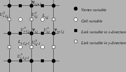
Consider a rectangular mesh such as that of Fig. 1, consisting of N_x x N_y cells, with mesh spacings a_x and a_y. Any numerical method is defined by the (finite) unknowns of the method plus the equations relating these unknowns. In the $\psi U$ method the fundamental unknowns are three complex arrays:

• $\psi_{i,j}$, with $1 \le i \le N_x+1$, $1 \le j \le N_y+1$, associated to the nodes (or vertices) of the mesh. The value of $\psi_{i,j}$ approximates that of the order parameter at position (x_i,y_j). In the program, the corresponding array is F(i,j).
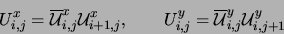
• U^x_i,j (link variable in the x-direction, with $1 \le i \le N_x$, $1 \le j \le N_y+1$, associated to the horizontal links (cell edges) of the mesh. The value U^x_i,j approximates that of $\exp (- \imath \int_{x_i}^{x_{i+1}} A_x (\xi, y_j) ~d\xi )$.
• U^y_i,j (link variable in the y-direction, with $1 \le i \le N_x+1$, $1 \le j \le N_y$, associated to the vertical links of the mesh. The value U^y_i,j approximates that of $\exp (- \imath \int_{y_j}^{y_{j+1}} A_y (x_i, \eta) ~d\eta )$.

To derive the discrete equations it is useful to notice that, from the definition of the link variables, discrete analogs of ${{\cal{U}}}^x$ and ${{\cal{U}}}^y$ from (1)-(2) can be defined at the nodes as

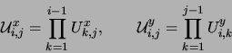$${\cal{U}}_{i,j}^{x} = \prod_{k=1}^{i-1} U_{k,j}^{x}, \qquad {\cal{U}}_{i,j}^{y} = \prod_{k=1}^{j-1} U_{i,k}^{y}$$ (8)

which leads to

$$U_{i,j}^{x} = {\overline {\cal{U}}}_{i,j}^{x} {\cal{U}}_{i+1... ...j}^{y} = {\overline {\cal{U}}}_{i,j}^{y} {\cal{U}}_{i,j+1}^{y}$$ (9)

Figure 1: Scheme of computational cells defining the numbering of discrete variables.