External boundary conditions

Equations (18)-(20) are not defined for boundary nodes or links. We adopt the usual methodology of constraining boundary values of the unknowns to satisfy first order approximations of the boundary conditions.

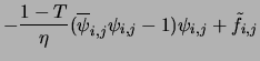
If the boundary is aligned with the y-axis, the zero-current condition implies $(-\imath \partial_x - A_x) \psi = 0$ or, equivalently, $- \imath \,{\overline {\cal{U}}^x} \partial_x ({\cal{U}}^x \psi) = 0$. For the order parameter at i=1 (West boundary) and i=N_x+1 (East boundary) this is implemented as

$$\psi_{1,j} = U^x_{1,j} \psi_{2,j} \qquad \psi_{N_x+1,j} = {\overline U^x}_{N_x,j} \psi_{N_x,j}$$ (22)

Similarly, for the South (j=1) and North (j=N_y+1) boundaries the expression is

$$\psi_{i,1} = U^y_{i,1} \psi_{i,2} \qquad \psi_{i,N_y+1} = {\overline U^y}_{i,N_y} \psi_{i,N_y}$$ (23)

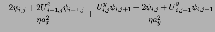
For the link variables, it remains to define how to update the values of those on the boundary. Notice that, for cells with two edges on the boundary only the product of the two link variables has numerical consequences, since it is the total circulation of the vector potential around the cell that propagates inside the computational domain. We have thus one unknown for each cell on the boundary, with the other three link variables already calculated from Eq. (19) or Eq. (20). Let H_e be the applied field and let the cell (i,j) be at the boundary. From

$$L_{i,j} = U^x_{i,j} U^y_{i+1,j} {\overline U}^x_{i,j+1} {\overline U}^y_{i,j} = \exp \left ( - \imath a_x a_y H_e \right )$$ (24)

the unknown link variable is readily obtained.

Remark: Notice that it is not difficult to obtain second order approximations to the boundary conditions that would preserve the accuracy of the scheme of Eqs. (18)-(20). Taking as example the East boundary (i=N_x+1), a second order approximation of the zero-current condition leads to

$$\partial_t \psi_{i,j} \frac {- 2 \psi_{i,j} + 2 {\overline U}^{x}_{i-1,j} \psi_{i-1,j}}... ...si_{i,j+1} - 2 \psi_{i,j} + {\overline U}^{y}_{i,j-1} \psi_{i,j-1}}{\eta a_y^2}$$ =

$$- \frac{1-T}{\eta} ({\overline \psi}_{i,j} \psi_{i,j} - 1) \psi_{i,j} +\tilde{f}_{i,j}$$ (25)

This coincides with (18) under the assumption $U^x_{i,j}\psi_{i+1,j}={\overline U}^x_{i-1,j} \psi_{i-1,j}$, or, equivalently, ${\cal{U}}^x_{i+1,j}\psi_{i+1,j}={\cal{U}}_{i-1,j} \psi_{i-1,j}$ (a second order approximation to $\partial_x ({\cal{U}}^x \psi )=0$). One can proceed analogously with the link variables. This variant has not yet been adopted in practice, though it deserves at least a try.