Next: External boundary conditions
Up: Numerical method
Previous: Numerical method
In the following, discrete approximations for each term of
(3)-(4) are derived, maintaining second
order accuracy in space.
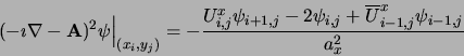
- Term
-
 : From the
identity
: From the
identity
a second order approximation at (xi,yj) reads
 |
(10) |
- Term
-
 : It is readily
approximated by
: It is readily
approximated by
 |
(11) |
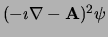
- Term
-
![${\rm Re} \left[ {\overline \psi}
\left( -\imath\nabla -{\bf A}\right) \psi \right]$](img52.png) :
From the identity
:
From the identity
it follows that
 |
(12) |
and analogously for the y component.
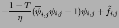
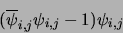
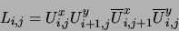
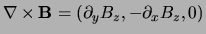
- Term
-
 (
(
 )
:
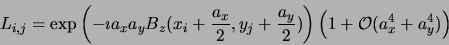
We introduce as auxiliary variable
)
:
We introduce as auxiliary variable
 |
(13) |
In the program, the
corresponding array is bloop(i,j).
From this and Stokes' identity it follows that
 |
(14) |
so that, since
 and thus
 ,
we can use the approximations
,
we can use the approximations
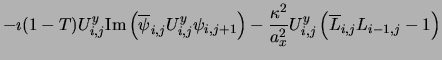
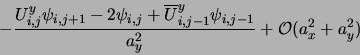
- Term
-
 :
From
:
From
it follows that
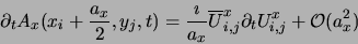 |
(17) |
and similarly for
 .
.
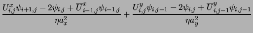
Collecting the previous results, the numerical method for interior
nodes reads:
Finally, a simple forward-Euler scheme is adopted to discretize
the time variable with step  ,
namely
,
namely
 |
(21) |
and analogously for Uxi,j and Uyi,j.
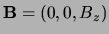
Notice that the random force  is also treated as a
vertex variable.
At each vertex it is selected from a
Gaussian distribution with zero mean and standard deviation
is also treated as a
vertex variable.
At each vertex it is selected from a
Gaussian distribution with zero mean and standard deviation  given
by
given
by
as done in Ref. [5].
Next: External boundary conditions
Up: Numerical method
Previous: Numerical method
Gustavo Carlos Buscaglia
2000-07-20