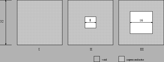
We detail in the following a few numerical examples. These depict some of the typical phenomena that occur in superconducting systems and how they are modeled by the described method. The reader is referred to [7] for an application of the model to the study of vortex arrays in superconducting thin films. It is also possible to extend the formulation to consider d-wave superconductors, as has been done in [10,11].
Consider first the case of a square sample with no hole (case I, see
Fig. 3), with
dimensions
![]() .
We use, with the units
defined in Section 1,
ax = ay = 0.5,
.
We use, with the units
defined in Section 1,
ax = ay = 0.5, ![]() ,
,
![]() and T=0.5, with
a noise constant of E0=10-5. With these definitions
Hc1=0.04 and Hc2=0.5 for the bulk material, while
Hc3=0.85 for a semi-infinite domain.
Numerical
limitations arise in the choice of the time step due to the
forward-Euler treatment of the equations. A practical rule for
time step selection is
and T=0.5, with
a noise constant of E0=10-5. With these definitions
Hc1=0.04 and Hc2=0.5 for the bulk material, while
Hc3=0.85 for a semi-infinite domain.
Numerical
limitations arise in the choice of the time step due to the
forward-Euler treatment of the equations. A practical rule for
time step selection is
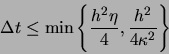 |
(33) |
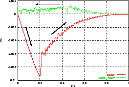
This case is particularly simple and runs at about 2500 steps per
minute on a personal computer. The magnetization curve that is obtained
can be seen in Fig. 4 (a). For applied fields
smaller than He =0.203 the sample remains in a Meissner state, but at
this field an instability develops that leads to the entrance of four
vortices with the consequent jump in the magnetization. Similar
vortex-entrance events occur at He = 0.216 (8 vortices),
0.252 (4 vortices), 0.270 (4 vortices), 0.288 (4 vortices),
0.312 (4 vortices), etc. In Figs.
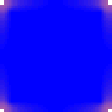
5 we show the
distribution of the modulus of the order parameter on the sample
for several values of the applied field. It can be observed that
the arrangement of the vortices is strongly affected by the finite
size of the sample and its square symmetry. Larger samples allow for
the obtention of hexagonal vortex lattices (an example can be
seen in Fig. 6). Also notice that for
He > 0.4 the superconductivity is strongly depressed in the
sample's interior, but recovers near the boundary. This gradually
leads, for ![]() or greater, to surface superconductivity in
a layer a few coherence lengths thick. The corners always remain
the points where the order parameter is maximal.
or greater, to surface superconductivity in
a layer a few coherence lengths thick. The corners always remain
the points where the order parameter is maximal.
The series of minima in the magnetization curves deserve special attention. Similar extrema were measured by Guimpel et al [12] and by Brongersma et al [13]. A related phenomenon was reported by Hünnekes et al [14]. In [7] it was argued that the minima reflect the magnetization behavior of the superconducting sheet at the sample surface and not rearrangements in the vortex lattice (which do occur). The simple case reported here confirms this argument, since minima extend far beyond Hc2 (He=0.5) and must thus come from a surface effect.
|
|
In Fig. 4 (a) the hysteretic behavior of the system
is clearly observed. Beginning at the calculated solution for
He=1, negative increments in the applied field
were imposed to show the hysteresis. Some snapshots of ![]() can be seen in Fig 7. For any given field,
there are many more vortices in the sample when the applied field
is decreasing than increasing. The lower (absolute) values in the
magnetization suggest a smaller barrier for vortices
to leave the system than the barrier for vortices to enter the
system. The results are however not conclusive since in the
simulation the rate of change of the applied field is rather
high and time-dependent terms play a role. The three vortices
in Fig. 7 (l), for example, leave the
sample if the field is kept constant at He=0 during another 35000
time steps.
can be seen in Fig 7. For any given field,
there are many more vortices in the sample when the applied field
is decreasing than increasing. The lower (absolute) values in the
magnetization suggest a smaller barrier for vortices
to leave the system than the barrier for vortices to enter the
system. The results are however not conclusive since in the
simulation the rate of change of the applied field is rather
high and time-dependent terms play a role. The three vortices
in Fig. 7 (l), for example, leave the
sample if the field is kept constant at He=0 during another 35000
time steps.
Consider now a hollow sample. Let the hole be a
centered square, with dimensions
![]() (case II), or
(case II), or
![]() (case III). The
same process of increasing and decreasing the applied field
as before is conducted. The
magnetization curves can be observed in Fig. 4 (b).
Essentially the same structure as before arises, but at zero
field in case II and III there remain fluxoids ``trapped'' in the
sample. These fluxoids (5 for case II and 13 for case III) do
not leave the sample if the simulation is continued keeping
He=0 for as many as 106 additional time steps.
(case III). The
same process of increasing and decreasing the applied field
as before is conducted. The
magnetization curves can be observed in Fig. 4 (b).
Essentially the same structure as before arises, but at zero
field in case II and III there remain fluxoids ``trapped'' in the
sample. These fluxoids (5 for case II and 13 for case III) do
not leave the sample if the simulation is continued keeping
He=0 for as many as 106 additional time steps.
Vortex arrangements are also different, as shown in Figs. 8-9. It is interesting to remark how the first four vortices that enter the system are ``captured'' by the hole in case II, and similarly for the first sixteen ones in case III. In Fig. 8 (b) the instant before the capture has been depicted, and similarly in Fig. 9 (f). The dynamics can be better grasped looking at animated sequences. Some are available at the same webpage mentioned above, or can be reproduced with the program in a few hours of CPU time.
We end up here the example section, since it is not the purpose of this article to discuss particular applications of the proposed method but rather to illustrate some physically interesting cases that can be simulated with the program.
|
|
 (a)
(a)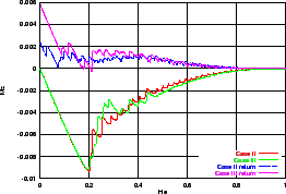 (b)
(b) (a)
(a) (b)
(b) (c)
(c)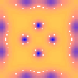 (d)
(d)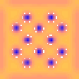 (e)
(e)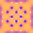 (f)
(f)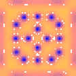 (g)
(g)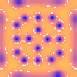 (h)
(h)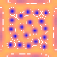 (i)
(i)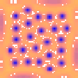 (j)
(j)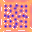 (k)
(k)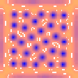 (l)
(l)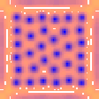 (m)
(m)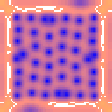 (n)
(n)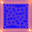 (o)
(o)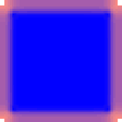 (p)
(p)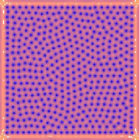
 (a)
(a)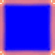 (b)
(b)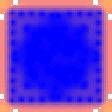 (c)
(c)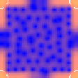 (d)
(d)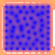 (e)
(e)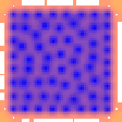 (f)
(f)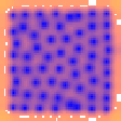 (g)
(g)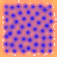 (h)
(h)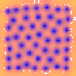 (i)
(i)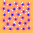 (j)
(j)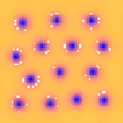 (k)
(k)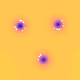 (l)
(l)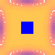 (a)
(a)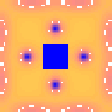 (b)
(b)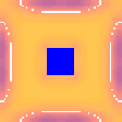 (c)
(c)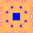 (d)
(d)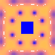 (e)
(e)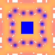 (f)
(f)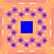 (g)
(g)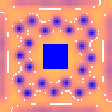 (h)
(h)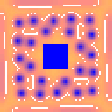 (i)
(i)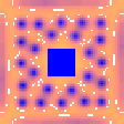 (j)
(j)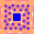 (k)
(k)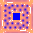 (l)
(l)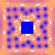 (m)
(m)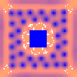 (n)
(n)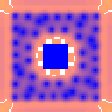 (o)
(o)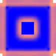 (p)
(p)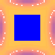 (a)
(a)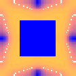 (b)
(b)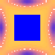 (c)
(c)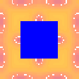 (d)
(d)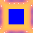 (e)
(e)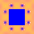 (f)
(f)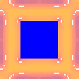 (g)
(g)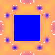 (h)
(h)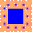 (i)
(i)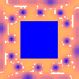 (j)
(j)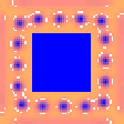 (k)
(k)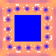 (l)
(l)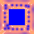 (m)
(m)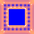 (n)
(n)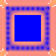 (o)
(o)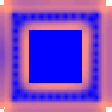 (p)
(p)